Tampilkan postingan dengan label Oseanografi. Tampilkan semua postingan

Sabtu, 05 Februari 2022

Menentukan variabel yang berpengaruh menggunakan Principal of Component Analysis (PCA)

Pada berbagai riset di bidang perikanan dan kelautan, kadang peneliti dihadapkan dengan situasi dimana data pengukuran kualitas perairan yang telah diambil sangat banyak namun kesulitan untuk menentukan parameter atau variabel mana yang paling mempengaruhi kondisi lingkungan/sampel dari fenomena riset yang ditemui. Salah satu tools yang mudah dan dapat diaplikasikan ke dalam riset tersebut adalah menggunakan metode Principal of Component Analysis (PCA).

PCA atau dalam bahasa indonesia disebut sebagai analisis komponen utama, merupakan suatu metode dalam statistika yang dapat digunakan untuk menyederhanakan data dengan mentransformasikannya secara linier membentuk sistem koordinat dimana masing-masing kuadran memiliki varians yang spesifik. Di dalam metode PCA, data dibagi menjadi beberapa kluster untuk memudahkan interpretasi hasil, yang secara umum teknik ini mirip sekali dengan teknik clustering. Kelebihan lain dari metode PCA adalah tidak memerlukan dependent variables, sehingga interpretasi yang diberikan mirip dengan teknik clustering K-means menggunakan pendekatan unsupervised learning.

Secara umum, PCA memberikan hasil akhir yaitu dapat mengetahui dan menganalisis faktor mana yang paling berperan untuk menjelaskan fenomena dalam dataset dengan tetap menjaga sifat-sifat data (variansi maksimum).

Beberapa aplikasi yang dapat digunakan untuk menggunakan pendekatan metode ini diantaranya adalah SPSS, MiniTab, MS Excel dan XLSTAT. Meskipun memiliki tampilan yang berbeda-beda, pada umumnya akan memiliki hasil pembacaan yang sama; yaitu data yang berada di dalam satu kuadran memiliki karakteristik yang sama, sehingga data tersebut merupakan data yang paling mempengaruhi kondisi fenomena yang diteliti. 

Sebagai contoh, kita misalkan seorang peneliti ingin mengetahui perbedaan karakteristik kepiting yang dibudidayakan di area pesisir (A), tambak darat dekat pesisir (B), muara (C), hingga laut lepas (D). Data yang diambil adalah sebagai berikut:


Data yang diambil masing-masing dua data panjang kepiting di 4 lokasi penelitian, dengan 5 pengukuran kualitas perairan. Selanjutnya, peneliti ingin mengetahui faktor kualitas perairan apa yang paling berpengaruh terhadap perbedaan panjang kepiting di berbagai lokasi tersebut.


Analisis PCA mengelompokkan pH dan suhu ke dalam satu kuadran, DO dan salinitas ke dalam kuadran panjang kepiting, serta TSS sebagai variabel yang tidak berkaitan dengan variabel-variabel lainnya. Sehingga, secara umum, menurut analisis PCA, perbedaan panjang kepiting, sangat dipengaruhi oleh kadar DO dan salinitas yang tersedia di perairan tersebut.

Adakah terumbu karang hidup di KEE Mangrove Ujungpangkah Gresik??? Studi kasus menggunakan pendekatan inderaja

Suatu ketika saya terlibat dalam kegiatan yang memerlukan analisis lokasi secara menyeluruh di area yang saat ini ditetapkan sebagai Kawasan Ekosistem Essensial (KEE), tepatnya di Kecamatan Ujungpangkah Kabupaten Gresik Jawa Timur. Area yang dilindungi mencakup tiga desa di kecamatan tersebut, meliputi Desa Banyuurip, Desa Pangkahwetan, serta Desa Pangkahkulon. Berbagai flora dan fauna yang spesifik menghuni area tersebut. Adanya burung-burung migrasi, mangrove, kepiting, kerang-kerangan, blodok, dsb; dimana area tersebut berdampingan erat dengan area kerja mayoritas penduduk disana, yaitu pembudidaya dan penangkapan produk perikanan.

Dikarenakan perlunya mengambil kesimpulan secara menyeluruh terhadap kondisi perairan disana, maka dicobalah untuk menganalisis melalui pendekatan penginderaan jauh. Citra satelit yang digunakan adalah Landsat dan MODIS. Peta yang kami gunakan adalah peta KEE MUP Gresik (Data tidak dilampirkan).

Beberapa hasil analisis (Kandungan klorofil-A dan suhu permukaan laut/SPL) dapat dilihat pada gambar-gambar berikut ini.


Kadar klorofil-A pada Bulan Januari-Maret 2021 berkisar antara 4-9 mg/L dengan suhu permukaan laut 30-36C. Kondisi ini mengikuti arah pergerakan angin pasat barat yang bergerak dari arah barat ke timur perairan Laut Jawa. Hasil analisis kualitas perairan secara keseluruhan tidak saya bahas disini.

Satu hal yang menarik adalah saat saya mencoba mengamati keberadaan terumbu karang di KEE MUP menggunakan data landsat Oktober 2020. Data menunjukkan terumbu karang tersebar merata di area Pangkah, padahal area tersebut memiliki tingkat sedimentasi yang cukup tinggi dari muara, yang secara umum tidak cocok untuk menjadi habitat terumbu karang. Selain itu, beberapa jenis ikan yang ditemukan bukan merupakan ikan-ikan spesifik penghuni terumbu karang.


Menurut data citra satelit, terumbu karang ini tersebar di area KEE barat dan timur. Akan tetapi, di lapangan, belum ada penelitian yang menunjukkan keberadaan terumbu karang di titik tersebut. Sudah dilakukan pula wawancara dengan penduduk sekitar meskipun dinyatakan di titik-titik tersebut diduga tidak ada terumbu karang. Saya juga sudah bertanya kepada beberapa peneliti dan pemerhati di bidang biologi laut & inderaja serta mendapatkan jawaban serupa, "Memangnya ada terumbu karang di Kec. Ujungpangkah Gresik?" 
Pendekatan ini saya coba ulangi dengan menggunakan variasi beberapa komposisi band dan hasil masih menunjukkan keberadaan terumbu karang di titik-titik tersebut. Memang, salah satu kelemahan dari citra ini adalah tidak dapat membedakan terumbu karang yang mati dan hidup. Dan hingga saat ditulisnya artikel ini, saya belum mengetahui adanya citra satelit yang bisa menandai dan membedakan lokasi terumbu karang mati dan hidup tanpa adanya ground checking ke lapangan. Meskipun, jika kita hubungkan dengan data klorofil-A dan SPL pada titik lokasi, seharusnya tidak cocok untuk habitat terumbu karang.


Hal yang menarik lagi adalah setelah ditelusuri menggunakan jalur darat, di salah satu area KEE terdapat hamparan terumbu karang yang kondisinya sudah mati. Namun, area tersebut justru tidak ditandai sebagai terumbu karang dalam citra satelit.


Agaknya, diduga ini adalah sedikit kekurangan dari citra satelit landsat ETM yang memberikan hasil bias antara terumbu karang dengan substrat keras non karang (Hickey dkk, 2020) sehingga perlu dilakukan reduksi data spasial di dalam pengolahan data citra (Gapper, 2019). Tetapi, overall memang inderaja hanyalah sebuah tools, bukan untuk menunjukkan hasil yang konkrit. Perlu dilakukan pengecekan secara in situ sebelum dipastikan data tersebut valid. Itulah pentingnya pengecekan secara langsung dan pendekatan inderaja dipadukan secara bersama untuk meneliti berbagai fenomena didalam pengembangan ilmu pengetahuan bidang perikanan-kelautan. Kesimpulan lainnya, bisa pula metode ini tetap dilakukan namun menggunakan citra satelit lain yang memiliki ukuran piksel lebih tinggi dengan area luasan yang lebih spesifik untuk mengetahui kebenaran adanya terumbu karang di lokasi tersebut serta menggunakan data-data lain seperti kisaran kualitas air yang cocok untuk pertumbuhan terumbu karang atau data sekunder ikan-ikan yang ditemukan di area tersebut untuk memastikan keberadaan terumbu karang hasil citra satelit.


*Sengaja data inderaja terumbu karang, SPL, dan klorofil saya munculkan karena memang hanya sekadar asumsi dan opini, dikarenakan ketertarikan saya dalam mempelajari biologi kelautan dengan keterbatasan waktu dan tenaga untuk membuktikan fenomena ini. Saya merasa sayang sekali jika data-data yang sudah dibuat dan dianalisis ini dihapus dan dibuang begitu saja.

Referensi:
Hickey SM., dkk. 2020. Between a Reef and a hard Place: Capacity to Map the Next Coral Reef Catastrophe. Front. Mar. Sci. https://doi.org/10.3389/fmars.2020.544290
Gapper JJ. 2019. Bias Reduction in Machine Learning Classifiers for Spatiotemporal Analysis of Coral Reefs using Remote Sensing Images. Chapman University. https://digitalcommons.chapman.edu/cgi/viewcontent.cgi?article=1001&context=cads_dissertations

Selasa, 10 Oktober 2017

Hypertrophication: The Good and The Bad Sides. Its Consequences to Global Warming

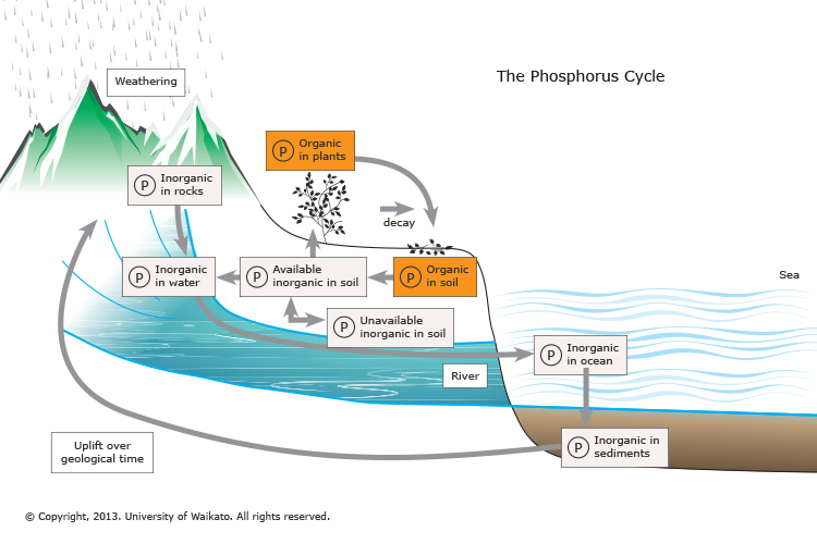
It is a well known that the excess amount of nutrients (especially because of algae) in the waters are known as hypertrophication/eutrophication. The water condition with unbalance nutrients caused algal blooming. In fact, the composition of nitrogen (N), phosphorus (P), and silicon (Si) should be 16:1:1. Therefore, the imbalance proportion of these substances lead to an alteration of plankton succession process. N and P are important elements to algae. On phosphorus cycle, the organic N compound from death plants and animals was decomposed by decomposer to be anorganic phosphorous; dilute inside soil water or sea water and settle on sediment. After being eroded, this material would be permeated by plants and phytoplanktons in oganophospate form. Nitrogen cycle is not much different. In this cycle, there is nitrogen fixation process from atmosphere to the land, settled on soil. Mineralization as well as nitrification-denitrification process are also occur.
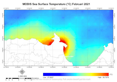
If these natural mechanisms work in harmony with balance composition, there would not be any conflicting matters. However, since the 20th century, this equivalence nutrient composition in the water, especially marine environment, were transformed differently. The N and P contents were increased, waters became eutrophic due to phosphorus and nitrate total concentration were 35 to 100 µg/L. Fish and other biota in the ecosystem chains were lost resulted in water ecosystem balance distraction.
People assumed domestic wastes from land is the main reason of this incidents. Well, yes it is. Long term investigation on various lakes in the world delivered conclusion that phosphorus is the main element neeeded by primary nutrient producers (C, N and P) on hypertrophication process. Results showed that while C and N were added on the lake, the algal blooming was not occured. Nevertheless, in another lake, the addition of P in the water (phosphate and slight amound of nitrate) is able to induce blooming. So why this phosphate is abundant?
Generally, 10% of phosphate was originated from natural water process, 7% from industry, 11% from detergent, 17% from agricultural fertilizer, 23% from human wastes and 32% from husbandry wastes. Thus, all organisms on the land donate these phosphates. Higher population generated to higher phosphate thrown away in the water and marine environment, resulted in higher hypertrophication possibility.
The interesting point is hypertrophication create a significant impact in ocean and coastal environment. On nitrification-denitrification process, the decomposing step by Nitrococcus, Nitrosomonas and Nitrobacter bacteria occur aerobically resulted in oxygen depletion. Decomposing products will formed mineral mud and create silting in the water. Another consequences are water colour was greenish, smells not good (ammoniac stink outcome from aerobic decomposition) and water turbidity. The results are clear, ecosystem is destroyed and all organisms are dead.
Water hyacinth (Eichhornia crassipes) and harmful blue-green algae (Cyanobacteria) will invade aquatic environment. The latter contains specific toxin which able to bring serious poisoning to human and animal. The water quality becomes zero. On social-economic side, hypertrophication eliminates conservation worth, aesthetics, recreational and tourism, thus, require much funding to solve it.
The-phosphorus-cycle20160510-28982-4ca08w.jpg
Developed countries, such as USA and european countries, already had proposed hypertrophication as environmental agenda with creating a special committees to find the solution of environmental pollution. In principal, they are very restrictive to phosphate amount in the aquatic and marine environment. They also labeled phospate free or environmental friendly to daily home products and reduce phospate and nitrate compound by specific treatment series. In Chinese and Korea, they use active bacteria—algae eaters—to clean the pollution.
In the relation with global warming, hypertrophication is two sides of blade, connecting each other with positive and negative impact. Cyanobacteria has chemical protection such as toxic and bioactive substances which is able to attack grazers: zooplankton Daphnia spp and other competitors. Its tolerance to ultraviolet radiation (containing shironine, mycosporine-glycerine, poryphyra-334 and scytonemin) generates it to live in high illumination, tend to blooming on warm temperature. Of course, the existance of global warming lead to the increasing of hypertrophication. These resulted in algal growth period becoming longer.
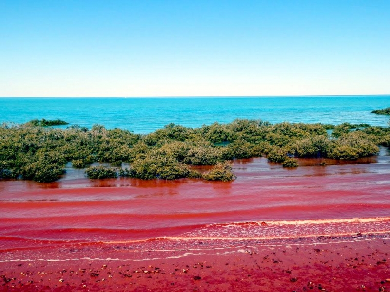
The algal blooming is effecting its toxic blooming. In Pensacola Bay, the abundance of Cyanobacteria Synechoccus at estuarine water created a red tide and induced a massive death of zooplankton and other biota. In Canada and Alaska coastal area, Cyanobacterial blooming leaded to new diseases on human, Paralytic Shellfish Poisoning (PSP), resulted in gastrointestinal and neurologic disturbance because of consuming toxic shellfishes. The exacerberated situation was if carbon dioxide was absorbed too much, seawater will became more acid. Shellfishes are filter feeder organisms which live in photic abyssal zone. They need calcium carbonate (CaCO3) to create their shell. The acid environment will easily make them absorbed it to strengthen their shell and make them much more poisonous.
gnb.jpg
Scientist has found carbon absorption of algae is much more bigger than carbon absorption of tree. Algae was also found as the first plant in the world that could produce oxygen. Surprisingly, European scientists incorporated in EIFEX (European Iron Fertilization Experiment) was deliberately inserted iron substance (Fe) to combine with phosphorus so that the photosynthesis process will be bigger and algal blooming will be occured. When the Antarctic was left to its natural mechanism, algae grow reasonably. After Fe addition, the hypertrophication was happen and increased algal photosynthesis. During this step, carbon dioxide from the atmosfer was absorbed through the excess algae. Furthermore, when these algae died or being eaten, carbon will be settled in the base of ocean, brought greenhouse gases within, reduced the temperature, and cooling the world!
Like Cyanobacteria, on Arctic Ocean, the one-celled-algae phytoplankton are able to soak 45 billion ton of carbon dioxide every year and deliver half of oxygen supply in the world. The first phytoplankton blooming indicated 400 ppm carbon dioxide reduction in the air, reduce a slight global warming in the world. In fact, the old satellite imagery described 10 times lower in investigating this phenomena; suggesting that algal abundance below the ice layer of Arctic Ocean was even more. In 2010, NASA found 100 km of phytoplakton under the ice near Alaska. Beforehand, the scientists assumed that the ice was blocking sunlight, which is needed for plants to grow on. But currently, they hyphotized that ice coloumn was melting and the sunlight was concentrated like magnifying glass. The global warming causing phytoplankton bloom two times faster. Although algae (phytoplankton in it) are able to absorb carbon massively, they also have higher effects for migrating birds and whale or the other marine organisms if left longer.
The hypertrophication problem is a dilemma. Although the harmful algae is only 2% from all species, they abundance will disturb food chain equilibrium. Its so irony, without algae, people cannot live constantly. Algae is everywhere, not only in the marine or other water environment. All living creatures including human need a healthy oxygen produced by algae. Nevertheless, their blooming and global warming existance endanger all living organisms in the world. Therefore, this obstacle need a continuous action to finish the problem. Reduce human pollution, reduce inorganic wastes, buy environmental friendly products, cultivate several plants on every houses, reduce greenhouse, are adequate action to diminish the global warming and algal blooming. Lastly, hypertrophication phenomena, wherever it is, of any size, will deliver a great influence for natural ecosystem and human life. LET’S SAVE THE WORLD!!!

Selasa, 05 September 2017

Medaka, A Monitoring Agent of Marine Environmental Pollution


The book our stolen future brought world-wide attention to scientific discoveries about a facts that common contaminants can interfere with organism developments, especially endocrine disruption. At sea, toxic chemicals is one of the most dangerous disturbance to marine population. Do you still remember minamata tragedy? Aside from hundreds of human, all of fishes were also died and floated because of dramatic increase of mercury’s poison at Minamata Bay, 1956.
At this time, the scientist are monitoring water environment to control the toxic pollution at coastal marine environment. Physical and chemical parameters were measured, and medaka fish was also used to examine the pollution degree & its bioavailability.
Medaka (Oryzias sp.) are actinopterygii or ray-finned fish with the average body length were 3 cm. This genus comprises more than 14 species, with the java medaka (O. javanicus-Bleeker, 1854) is the most highly adaptable to different salinity (can live in fresh water, brackish water, as well as salt water) among other Oryzias species. On meristic experiments, the number of dorsal fin were 6-7, anal fin 20-25 and caudal fin were 5-6.  They eat artemia, insects, tubifex worms and protozoa.
map_of_Oryzias_javanicus
Java Medaka are widely distributed in Asia, especially in Indonesia, Malaysia and Thailand and live in well defined habitat. They have a unique osmotic adaptation mechanism (enhances the capacity of Na+ and Cl secretion in ionocytes and hypoosmoregulatory ability while exist in seawater).  They live long-enough with short generation time (2-3 months, make them possible to obtain five generations a year) and available at all periods of the year. Medaka are also highly adaptable fish and stable in laboratory aquaculture. These create medaka as important fishes to monitor the pollution threat in the ocean.
Woo et al (2014) suggest that there is transcriptional changes caused by Bisphenol A (BPA) in java medaka. 533 genes of seawater, 215 genes of freshwater and 78 shared genes were changed significally their expression, which mainly involved in cellular and signaling pathway. These finding were also revealed the alteration of salinity as one of environmental stressor can potentially affect the toxicity, since transcriptional changes was also regulated differently under environmental salinity.
In addition, the induction of metallothionein (MT) chemical substance on juvenile java medaka are statistically significant with positive correlation with the cadmium level (Cd) in their tissues. 
Another study of low level Cd exposure (0.01-0.10 ppm) resulted in several development impairments to java medaka egg. Nevertheless, this impairment was significantly observed to eggs on low levels mercury (Hg), 0.01-0.02 ppm. Lower concentration of Hg were found to cause teratogenesis on java medaka. Although java medaka eggs successfully hatched 375.7 to 78.6% when exposed on high concentration of Hg, this fish is more sensitive to Cd exposure within the same concentration (successful rate 0-52.5%) (Ismail and Yusof, 2011).
As biological effect monitoring, Estrogenic chemicals (EI) and 17β-estradiol (E2) are a natural steroid hormone, detected in sewage treatment works effluents and estuarine water. They were known to cause induction of vitellogenin, the appearance of testis-ova in male fish and lead to endocrine disruption. Fortunately, based on Imai et al (2007) research, at very low concentration, 39-198 ng/L, java medaka will not be affected to these chemicals.
We expect that such continuous experimental is needed to understand the genetic variation and modification of java medaka after toxicology exposure, especially on offspring impact. The application of  experimental techniques to this fish would bring us new information to understand how medaka has developed diverse mechanisms to adapt in diverse environments as well.

References:
Colborn T, Dumanoski D, Myers JP. 1996. Our stolen future: Recent important scientific studies. http://www.ourstolenfuture.org/. Accessed on October 2017.
Fishbase. Oryzias javanicus. http://www.fishbase.org/summary/12254. Accessed on October 2017.
Imai S, Koyama J, Fuji K. 2007. Effects of estrone on full life cycle of java medaka (Oryzias javanicus), a new marine test fish. Environ Toxicol Chem. 26 (4): 726-731.
Ismail A., Yusof S. 2011. Effect of mercury and cadmium on early life stages of Java medaka (Oryzias javanicus): A potential tropical test fish. Marine Poll Bull. 63: 347-349.
Khododaust D, Ahmad I. 2013. Metallothionein-like protein levels in java medaka fish (Oryzias javanicus) exposed to different concentration of cadmium. Walailak J Sci & Tech. 11(10): 883-893.
Kudo A, Fujikawa Y, Miyahara S, Zheng J, Takigami H, Sugahara M, Muramatsu T. 1998. Lessons from minamata mercury pollution, Japan—After a continuous 22 years of observation. Wat Sci Tech. 38(7): 187-193.
Miyanishi H, Inokuchi M, Nobata S, Kaneko T. 2016. Past seawater experience enhances seawater adaptability in medaka, Oryzias latipes. Zoological Lett. 2(12): 1-10.
Woo S, Denis V, Yum S. 2014. Transcriptional changes caused by bisphenol A in Oryzias javanicus, a fish species highly adaptable to environmental salinity. Mar drugs. 12: 983-998.
First picture: http://3.bp.blogspot.com/_58yBWvhQZ-g/Sid2jPsNWaI/AAAAAAAAAEA/E0Xz78PVIqI/s1600/oryzias%252520javanicus%252520m-5

Rabu, 12 Juli 2017

Sea Horses, A Trusty Unique Partner

Do you often hearing about a pair of pigeon, when flown separated, they were able to find their own partner? Well, this phenomenon is not only exist in the air, we also have this couple in the sea! Yup, its sea horses couple.

These marine creatures have scientific name Hippocampus sp. with family Syngnathidae, kind of fish with a very particular form. Their body size are variated, 16 mm to 35 cm. This species has around 54 species in the world. The head of each sea horse is triangle, resembles of a real horse, with a long snout, forming 90º degree from its own body. The tail is elongated, curled, sharp in the end, and used as a holder.
Sea horses are spread in tropical and subtropical area in the world, commonly live in shallow water with seagrass, coral reef, seaweed, and mangrove habitat. Their lifespan are commonly 1 to 5 years. Sea horses have excellent eyesight and work independently on each side. These marine creatures eat almost anytime. They even don’t have any teeth or stomach,  the food just passes through their body very quickly. They eat plankton and able to comsume 3000 artemia everyday.
Sea horses are monogamy, they will just mating with only one partner in their life. Male seahorses were highly active and preferred a larger female, suggested the importance of the body size for a successful reproduction. To impress their partner, both individual male and female sea horses change colours to brighten. Although sea horses are not able to bend their own tail backwards, each couple are comfortably swim together in pairs by holding tails. They move vertically and swim slower than a slug, this also because of their straight body.
Similar to kangaroo, sea horses own egg sac on tummy to nurturing their kids. However, this egg sac exist on male. The other lovely thing is, during reproduction season, they performed a special dance! They did spawning use their own tail as hand to reach each other with this exclusive dance. After that, the anal fin of female sea horse entered to the male egg sac to transfered hundreds eggs to be fertilized by male. Until hatching time, the larva still kept in there and taken out when considerably strong enough.
Every time, especially during reproduction time, each sea horses couple will meet to confirm their eggs are well until hatching time and become adult sea horses. They love to holding tails each other and loyal to their ‘only one’ partner until death comes apart. What a remarkable lesson!

Reference:
1. Mattle B & Wilson AB (2009). Body size preferences in the pot-bellied seahorse Hippocampus abdominalis: choosy males and indiscriminate females. Behavioral Ecology and Sociobiology.
2. Ministry of Fisheries and Marine Affairs Republic of Indonesia. Guide Book to Sea Horses.

Selasa, 14 April 2015

Ocean Circulation

Proses Coastal upwelling akibat dari Ekman transport:

Upwelling di pesisir dapat disebabkan oleh sejumlah faktor. Dalam kebanyakan situasi upwelling terjadi karena didorong angin dan efeknya pada arus, pasokan nutrisi ditentukan oleh topografi rinci seperti kedalaman air dan bentuk garis pantai. Dalam situasi lain adalah karena respon terhadap variasi dalam arus yang ditemukan di luar laut pesisir dan karena itu independen dari kondisi angin pantai. Air yang naik dekat pantai harus dipasok dari daerah lepas pantai. Pada lapisan ini terjadi didalam lapisan batas bawah. Lapisan air lepas pantai tersebut berasal dari air pertengahan dalam. Pergeseran ini dikelola oleh gradien tekanan yang diarahkan dari khatulistiwa ke kutub dan hasil dari sirkulasi laut skala besar. Keseimbangan kekuatan di darat, gaya tekanan gradien ditentang oleh kekuatan Coriolis equatorward, tidak dapat beroperasi di sekitar lereng benua, sehingga gaya Coriolisnya nol. (Jones, 2010)


Kecepatan permukaan air laut saat ini mirip dengan yang telah diprediksi oleh Ekman bahwa arah arus permukaan tidak menyimpang dari arah angin. Namun, penyimpangan diprediksi kurang dari 45 derajat. Ada beberapa alasan untuk ini. Sebagai contoh, di banyak daerah laut terlalu dangkal, sehingga spiral penuh tidak dapat berkembang dan gesekan dengan dasar laut menjadi signifikan. Transpor ekman yang berhubungan dengan pergerakan angin memberikan kontribusi signifikan terhadap sirkulasi laut umum. ketika angin bertiup dari utara di sepanjang pantai barat di belahan bumi utara mereka mempercepat arus dekat permukaan ke arah selatan dan karena rotasi bumi arus ini cenderung membelok khatulistiwa menuju lepas pantai. Saat mereka membelok lepas pantai, air datang dari suatu tempat untuk mengisi air yang bergerak menjauh dari pantai. Sumber air yang umumnya dari bawah lapisan air yang bergerak lepas pantai, dan air ini datang ke permukaan dekat pantai. Karena air yang lebih dalam adalah bergerak ke atas ke permukaan dekat pantai, kita lihat proses sebagai upwelling - transportasi air vertikal ke atas (lihat skema di bawah). Air lebih mengandung nutrisi (nitrogen, fosfor, dan silikat) yang mendukung pertumbuhan tanaman mikroskopis (fitoplankton) di laut ketika mereka terkena sinar matahari. Alhasil saat upwelling yang signifikan terjadi di sepanjang pantai, kita sering melihat respon dalam pertumbuhan fitoplankton, seperti kita bahas ketika ada yang signifikan dari limpasan hujan. Sementara limpasan hujan kondusif tumbuhnya fitoplankton kelompok yang disebut dinoflagellata, upwelling cenderung untuk mendukung lebih kondusif untuk kelompok berkembang pesat fitoplankton diatom disebut (Cookes, 2010).
Menurut Brown (2004), di pesisir proses upwelling diubah dalam beberapa cara. Situasi laut dalam berlaku di mana lapisan cukup dalam untuk mengakomodasi permukaan lapisan Ekman, lapisan batas bawah dan lapisan geostrophic yang berada di antara kedua lapisan. Pengamatan menunjukkan bahwa pada daerah upwelling ketebalan lapisan Ekman sering lebih kecil daripada di lautan terbuka, mungkin karena upwelling termoklin membawa lebih dekat ke angin permukaan kemudian menghambat pencampuran melampaui kedalaman 20 - 30 m. Oleh karena itu cukup untuk memungkinkan situasi laut dalam untuk berkembang. Dengan kata lain, dalam kedalaman air melebihi 60 m upwelling terkuat dapat diharapkan terjadi ketika angin bertiup sejajar dengan pantai dengan garis pantai ke kiri (kanan) di belahan bumi (selatan) utara.Faktor kunci untuk upwelling adalah angin didorong dari lapisan transport Ekman relatif terhadap pantai. Kondisi upwelling optimum diperoleh ketika perbedaan transport Ekman dimaksimalkan, diarahkan lepas pantai dan normal dengan garis pantai. Lapisan transport Ekman akan lebih selaras dengan arah angin sebagai kedalaman air berkurang, arah angin yang paling menguntungkan bagi upwelling adalah sejajar dengan pantai tegak lurus pada perairan dangkal.
Ada dua jenis arus yang dihasilkan dari tekanan angin:
- Transpor ekman yang mengacu pada sudut kanan dari arah angin, dan:
- Arus geodesi, sebagai respon dari tekanan horizontal yang disebabkan tumpukan air secara terus menerus dari transpor ekman.


Macam-Macam Arus
1. Kuroshio Current


Arus Kuroshio adalah arus samudera dari timur laut hangat dari pantai Jepang. Biasa disebut sebagai arus teluk Pasifik atau Japan Current. Arus ini arus tercepat kedua setelah gulf stream. Sistem termasuk cabang mengikuti: Kuroshio, sampai 35 derajat N; Perpanjangan kuroshio memperluas ke timur ke dua cabang sampai 160 derajat garis bujur E; pasifik utara, kelanjutan ke timur, cabang ke selatan sejauh 150 derajat W; Kuroshio berasal dari bagian yang lebih besar dari Equatorial Utara yang membagi timur Pilipina. Kuroshio berada kira-kira 35 derajat garis lintang N. Ia berlanjut secara langsung sebagai arus hangat atau dikenal sebagai Kuroshio Extension. Air memasuki Kuroshio atas bidang luas, 621 mi (1,000 km), yang kemudian mempercepat dan memperkecil. 6 mi (1 km) kedalaman yang maksimum untuk 1,864 mi (3,000 km) sepanjang tepi barat Pasifik, antara Pilipina dan pantai timur Jepang. Kuroshio adalah arus samudera cepat. Setiap detik membawa beberapa 50 juta ton air laut masa lalu pesisir tenggara Jepang, menyamai volume untuk kira-kira 6,000 sungai seperti ukuran Danube atau Volga. Dampak besar di bidang perikanan lepas pantai dan pesisir berupa kuroshio Current memainkan peran penting dalam sirkulasi North Pacific Ocean. Dalam skala air yang besar mampu membawa sejumlah panas. Panas, yang dibawa ke utara oleh arus ini memiliki efek tentang iklim. (Tokarev, 2010)

Jumat, 13 Desember 2013

ESTIMASI DISTRIBUSI KLOROFIL-A DI PERAIRAN SELAT MADURA MENGGUNAKAN DATA CITRA SATELIT MODIS DAN PENGUKURAN IN SITU PADA MUSIM TIMUR

ESTIMASI DISTRIBUSI KLOROFIL-A DI PERAIRAN SELAT MADURA

MENGGUNAKAN DATA CITRA SATELIT MODIS DAN PENGUKURAN IN SITU
PADA MUSIM TIMUR

Nur Maulida Safitri[1], Bambang Semedi[2]
Ilmu Kelautan
ABSTRAK
Penelitian ini dilaksanakan di Selat Madura pada musim timur bulan Juni hingga September 2013. Tujuan dari penelitian ini adalah mengestimasi distribusi klorofil-a di Selat Madura menggunakan data citra satelit Aqua MODIS dan pengukuran in situ pada musim timur serta melakukan validasi nilai konsentrasi klorofil-a dari kedua data tersebut. Pengumpulan data pada penelitian ini dilakukan dengan metode penginderaan jauh, studi lapang dan laboratorium. Metode penginderaan jauh dilakukan dengan mengolah data klorofil-a dari Aqua MODIS. Data in situ diperoleh dengan cara mengukur parameter oseanografi (suhu permukaan laut, kedalaman, pH, oksigen terlarut, salinitas, kecerahan dan arus permukaan). Data laboratorium diperoleh dengan menganalisa konsentrasi klorofil-a menggunakan metode spektrofotometer. Hasil penelitian menunjukkan bahwa parameter oseanografi yang berkaitan dengan persebaran klorofil-a di perairan Selat Madura diantaranya adalah suhu permukaan laut, kecerahan, oksigen terlarut dan arus permukaan. Sebaran klorofil-a pada musim timur berkisar antara 0,022317 – 1,561958 mg/L dengan puncak sebaran tertinggi di bulan Juli yaitu berkisar antara 0,102566 – 1,561958 mg/L. Setelah dilakukan uji validasi uji R square, diperoleh nilai R square sebesar 80,14% sehingga dapat disimpulkan hasil analisa citra satelit berpengaruh besar terhadap hasil analisa in situ sebesar 80% dengan rata-rata konsentrasi klorofil-a hasil analisa citra 1,127181 mg/L dan rata-rata konsentrasi klorofil-a in situ 1,195664 mg/L. Kedua data memiliki nilai rata-rata pada rentang 1-1,5 mg/L sehingga dapat disimpulkan Selat Madura memiliki kandungan klorofil-a yang tinggi pada musim timur.
Kata Kunci : Klorofil-a, Aqua MODIS, Selat Madura, Validasi


ESTIMATION OF CHLOROPHYLL-A DISTRIBUTION IN THE STRAIT OF MADURA USING MODIS SATELLITE IMAGERY DATA AND FIELD MEASUREMENT
 ON THE EASTERN SEASON

Nur Maulida Safitri1, Bambang Semedi2
Marine Science
ABSTRACT
This research was carried out in the Strait of Madura on the eastern season, June to September 2013. The purpose of this research is estimating chlorophyll-a distribution in Madura Strait using Aqua MODIS image satellite data & field measurement on the eastern season and validating both chlorophyll-a values. Data were collected by remote sensing method, field and laboratory study. Remote sensing method performed in processing chlorophyll-a data from Aqua MODIS. Field data obtained by measuring the oceanographic parameters (sea surface temperature, water depth, pH, dissolved oxygen, salinity, brightness and surface current). Laboratoty study conducted by analyzing chlorophyll-a concentration using spectrophotometer method. The results showed that the oceanographic parameters related to the distribution of chlorophyll-a in the Madura Strait are sea surface temperature, brightness, dissolved oxygen and surface current. Distribution of chlorophyll-a in the eastern season ranged between 0,022317 mg/L – 1,561958 mg/L with the highest distribution in July that ranged between 0,102566 – 1,561958 mg/L. After the validation test is performed using R square test, the value of R square is 80,14% so it can be summed up that the results of satellite imagery analysis has huge influence against the results of data field, worth 80%, with the average concentration of chlorophyll-a from the image is 1,127181 mg/L and data field is 1,195664 mg/L. Both data have average value in the range of 1-1,5 mg/L so the conclusion is the Madura Strait has high chlorophyll-a concentration on the eastern season.
Key Word(s): Chlorophyll-a, Aqua MODIS, Madura Strait, Validation.


[1] Student of Marine Science’s Departement, FPIK, Brawijaya University
[2] Lecturer of Marine Science’s Departement, FPIK, Brawijaya University


Untuk mendapatkan penelitian lengkap mengenai abstrak ini silahkan menghubungi nurmaulidasafitri@gmail.com